相关性分析(by R)

#导入数据，第一行为表头，第一行是数据的话header = F
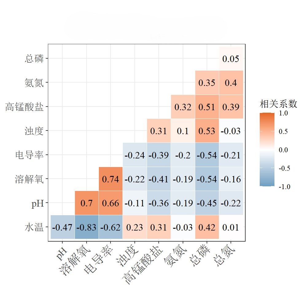
data1<-read.table('E:\\\数据\\all.txt',sep = "\t",encoding="UTF-8",header = T)

#多变量间相关性，提取data1第12列与第20列
data_cut<-data1[,12:20]
#剔除na值
data_cut<- na.omit(data_cut)
#查看数据属性
str(data_cut)
#如果数据不全是numeric则执行这一步
#for (i in 1:length(data_cut)) {
#  data_cut[,i]<-as.numeric(data_cut[,i])
#}

#计算所有数据间的相关系数（Pearson），保留3位小数
cordata <- round(cor(data_cut),3) 
#cov(x, y = NULL, use = "everything",method = c("pearson", "kendall", "spearman"))
#use是指定缺失值的处理方式，系统默认是use="everthing"和method="pearson"。

#用ggcorrplot进行画图
library(ggcorrplot)#788*668
p<-ggcorrplot(cordata,#数据
              title=paste0("XX参数相关性"),
              method = c("square"),#method, 指定可视化的形状，可以是circle圆形(默认)，square方形， ellipse, 椭圆形，number数值，shade阴影，color颜色，pie饼图。
              type=c("lower"),#type，指定显示范围，可以是full完全(默认)，lower下三角，upper上三角。
              hc.order = FALSE,#参数是否分层聚类
              outline.col ="white",#方块轮廓颜色
              ggtheme = theme_bw()+theme(plot.title = element_text(hjust = 0.5, size = 16,family="serif")),
              show.legend=TRUE,#图例显示
              legend.title = "相关系数",
              colors = c("#6D9EC1","white","#E46726"),#方块范围颜色
              lab = TRUE,#方块内数字
              #lab_col,#方块内颜色
              lab_size = 4)#方块内数字大小
p

#设置默认路径，后面图片保存在此路径
setwd("E:\\output\\相关性图")
jpeg(filename =paste0("output.jpg"),width=1000,height=1000,res=150,family ="serif" )#res 是指 PPI（Pixel Per Inch） ，即图像的采样率（在图像中，每英寸所包含的像素数目），越大线条越粗
p
dev.off()